Dr. Barry Haworth
University of Louisville
Department of Economics
Econ 301
Application of Indifference Curves: Lump Sum vs. Per Unit Taxes
Assume we have a new representative consumer, Marge Simpson, who derives different levels of utility from buying varying quantities of beer and pork rinds (QB = quantity of beer, QR = quantity of pork rinds).
Her utility can be calculated from the following utility function:
This utility function implies that her indifference curves, IC, have a slope that is nonlinear. That slope, called the marginal rate of substitution between beer and pork rinds, can be calculated by plugging different quantities into the equation below:
Let’s assume further that Marge faces the following prices and that she has the income given below as well.
Price of beer = $4
Price of pork rinds = $2
Income = $200
We can start our analysis by asking this question:
How many units of beer and pork rinds should Marge buy?
We know, from previous work/handouts, that there are two equations which will help us determine the answer to our question. Furthermore, we know that both must be true simultaneously. Those equations are:
(1) 4QB + 2QR = 200 (Marge must be somewhere on her budget constraint, BC)
(2) - 4/2 = - QR/QB (the slope of Marge’s BC must equal MRSB,R at equilibrium)
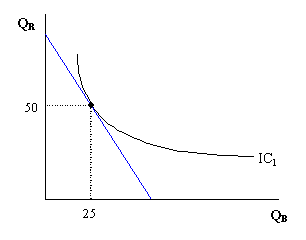
Solving (1) and (2) simultaneously (e.g. using algebraic substitution), we find that Marge will buy 25 units of beer and 50 units of pork rinds. Her indifference curve graph appears as:

Let’s assume that the government is considering two different types of tax. The first tax is a per unit tax. That is, a tax that is levied on the number of units of a specific good that are purchased by Marge. The second tax is a lump sum tax. That is, a tax of some fixed amount that does not correspond with the number of units Marge decides to buy of either good.
Suppose that a $1 per unit tax is levied on beer. This changes the actual price that Marge pays for each unit of beer. For each unit of beer that she purchases, she pays the sum of the equilibrium price and tax on that unit. For example, if the price is $4 per unit and the tax is $1 per unit sold, then Marge will pay $5 for each unit she buys. That changes the budget constraint equation (above) and, of course, the slope of the budget constraint as follows:
(1a) 5QB + 2QR = 200
(2a) - 5/2 = - QR/QB
Again, solving (1a) and (2a) simultaneously, we find that Marge will buy 20 units of beer and 50 units of pork rinds. The budget constraint shifts inward, and she moves to a new, lower indifference curve as follows:

We note that, with this per unit tax on beer in place, the government will raise $20 in tax revenue from Marge (i.e. Marge pays $1 tax for each of the 20 units she buys).
If the government decides to go with the lump sum tax, then Marge (and all other consumers) must pay (instead) a specific lump sum amount. It seems safe to assume that if the government raises the same amount of tax revenue from Marge with either tax, then the government will not have a preference as to which tax is used.
An important second question, however, is whether Marge has a preference. To answer this question, let’s assume that the government levies a lump sum tax of $20 on Marge (equal to the amount she’d pay with the per unit tax).
The new lump sum tax would reduce her Marge’s income by $20, but, unlike the per unit tax, will leave the price of beer unchanged. With her new, lower post-tax income ($180, instead of $200), Marge faces a new budget constraint. The budget constraint doesn’t change in slope, but does shift inward because of a change in each intercept. This is reflected in the following equations:
(1b) 4QB + 2QR = 180
(2b) - 4/2 = - QR/QB
Again, solving (1b) and (2b) simultaneously, we find that Marge will buy 22.5 units of beer and 45 units of pork rinds. On a graph, we see the budget constraint shift in parallel as Marge moves to a new, lower indifference curve (IC3):

The most straightforward method for determining whether Marge prefers one tax over the other is to calculate her utility in both situations. To do so, we utilize the utility function given at the beginning of this handout and then compare the utility associated with the per unit tax case and the lump sum tax case by plugging in the appropriate equilibrium values for QB and QR as follows:
Marge’s utility is higher when the government raises $20 in tax revenue from a lump sum tax than when the government raises $20 from a per unit tax.
Why do we get this result? In other material, we’ve noted that price changes have a dual effect on a consumer’s purchasing decision. There is both a change in relative prices, called the substitution effect, and a purchasing power change, called the income effect. When income changes, there is only one effect – the income effect. The per unit tax is comparable to a price change and so consumers react more with this tax than with the lump sum tax - when there is only a change in income. The difference in utility between these two cases represents a type of utility loss for Marge. Because deadweight loss arises when consumers substitute their consumption away from a particular good, the lump sum tax is thought to be more efficient, because the lump sum tax does not induce this kind of behavior (i.e. there is no substitution effect with a lump sum tax).