The marginal rate of substitution (which is the slope of Homer’s indifference curve) between beer and pork rinds is given in absolute value as:
Recall that this can be derived from Homer’s utility function. If we use a different utility function, then we get a different MRSR,B. Assume further that the price of beer is $4, the price of pork rinds is $2, and that Homer’s income is $200. We can obtain Homer’s budget constraint from this information, which we can rearrange as:
A consumer equilibrium occurs in the graph below at pt. X1, where the (blue) indifference curve is tangent to the (red) budget constraint.
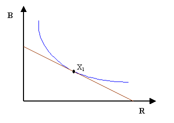
It is possible to calculate the quantities of beer and pork rinds at this consumer equilibrium. After doing so, we would find that B* = 25 units and R* = 50 units.
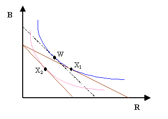
How is the graph above affected when the price of pork rinds increases from $2 to $4? This change is shown on the graph below. The budget constraint becomes steeper and Homer moves to a new (pink) indifference curve and a lower level of utility at pt. X2. If we calculate the new consumer equilibrium at pt. X2, we would get B* = 25 and R* = 25.

Notice, however, that the price change included two actions. The movement from pt. X1
to pt. X2 involved a change in the marginal rate of substitution (i.e. a change in the
slope of the indifference curve), and a change in utility (i.e. a change from the blue indifference
curve to the pink indifference curve). This is different from a change in income, which only
involves one change – a change in utility. These two actions form the analytical basis for what
we call the substitution effect and the income effect.
The Substitution and Income Effects
When prices rise, consumers lose purchasing power. What if the price of pork rinds goes up, but the government offers to compensate Homer for this loss of purchasing power. That is, Mayor Quimby offers to mail Homer a check, in an effort to keep Homer from feeling worse off. Homer still faces the higher pork rinds price, but doesn’t experience a change in utility. That is, for Homer to be no worse off after the price increase, the government check must be large enough to keep Homer on his original indifference curve.
If the government check allows Homer to remain on his original indifference curve, will he just return to pt. X1 and go back to buying 50 units of pork rinds? No. Even though Homer would return to his original indifference curve, he would also still face a different pair of prices. Therefore, we know that Homer must be located at a different point on that original indifference curve.
By taking the second graph above, and drawing a “hypothetical budget constraint”, we can find this new point. This new constraint must satisfy two criteria. First, the constraint must be parallel to the new prices (where beer and pork rinds each cost $4). Second, the constraint must be tangent to the original indifference curve.
The dotted line in the graph below satisfies these criteria, and so represents this new constraint. This line is tangent to Homer’s original indifference curve at pt. W. This point reveals the quantities of beer and pork rinds that Homer would buy after receiving his government check (the check that keeps his utility constant). Of course, in real life, Homer would never get a check from the Mayor, but we will use pt. W to distinguish between the two actions (or effects) we noted as occuring with every price change.
How much would Homer consume at pt. W?
The calculation is somewhat involved.
First, note that the slope of Homer’s new constraint is -1. Consequently, at pt. W,
the slope of his original indifference curve equals -1. If R/B = 1 at pt. W, then B = R at pt.
W also. That is, we can ascertain that Homer will buy an equal amount of beer and pork rinds at
pt. W.
Homer’s original level of utility is ![]()
(i.e. plug the original consumer equilibrium values of B = 25 and R = 50 into Homer’s utility function)
To maintain Homer’s original level of utility, then it must be true that:
That is, Homer will buy some combination of B and R that makes his utility function equal to ![]()
Recall that at pt. W, Homer will buy an equal amount of beer and pork rinds. Therefore, we can rewrite Homer's original level of utility (given above) as ![]()
Of course, the equation above tells us that B* is equal to ![]() , so given that B* = R*, we have the following:
, so given that B* = R*, we have the following:
The new (hypothetical) budget constraint would be given as 4B + 4R = 200 + DI,
where DI is the change in income necessary to keep Homer’s utility constant.
Plugging in B* and R* from the paragraph above, we find that DI = $82.84.
That is, if Homer receives a check for $82.84, then Homer can continue to receive
his original level of utility (i.e.
What are the substitution and income effects?
The income effect is measured as the quantity change attributed to moving from pt. W to pt. X2. Between these two points, only utility changes, there is no change in the
slope of the budget constraint. At pt. X2, Homer consumes 25 units of pork rinds.
The difference between pts. W and X2 is
Note that, like the substitution effect, there is a decrease in quantity within the income effect. Unlike the substitution effect, however, a negative relationship between price and quantity does not always arise within the income effect. For normal goods, the income effect reveals a negative relationship between price and quantity changes. That is, price increases lead to the income effect involving a decrease in quantity, and price decreases lead to the income effect involving an increase in quantity. Obviously, Homer considers pork rinds to be a normal good.
For inferior goods, we get the opposite result – the income effect involves a positive relationship between price and quantity changes. Any increase in price (decrease) would lead to the income effect yielding an increase in quantity (decrease).
Suppose the inferior good is highly inferior. For example, suppose we have a good where any small increase in price leads to a large, positive income effect. This would explain why a fairly large price change leads to an insignificant (overall) change in quantity. The inferior good’s large income effect moves in the opposite direction of the substitution effect, causing the overall change (i.e. the sum of the two effects) to be very small.
In some cases, if a good is inferior enough, the positive income effect may be so large that it leads to price increases (decreases) being accompanied by overall quantity increases (decreases). When this occurs, we are dealing with a special (and rare) type of good known as a Giffen good. Giffen goods are so inferior that the income effect overwhelms the substitution effect, leading to the perverse result described above – where there is an overall positive relationship between price and quantity changes.
![]() utils) even though pork rinds are $2 more expensive now.
utils) even though pork rinds are $2 more expensive now.
The two effects are separated by pt. W. As the quantity of pork rinds changes between pt. W and pt. X1 we observe the substitution effect. At pt. X1, Homer consumes 50
units of pork rinds. At pt. W, Homer consumes ![]() units of pork rinds (i.e. about 35.36 units).
The substitution effect associated with this price increase is represented by a decrease in
quantity. That is, the substitution effect reveals a negative relationship between the price
and quantity change. In fact, with every price change, we find this negative relationship
within the substitution effect.
units of pork rinds (i.e. about 35.36 units).
The substitution effect associated with this price increase is represented by a decrease in
quantity. That is, the substitution effect reveals a negative relationship between the price
and quantity change. In fact, with every price change, we find this negative relationship
within the substitution effect.
![]() , or about 10.36 units.
, or about 10.36 units.