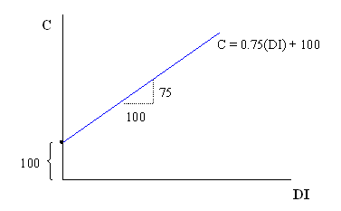
Before writing a consumption equation, we want to consider variable consumption expenditure a little more closely. More specifically, we want to know the rate by which this category varies. Letĺs assume that consumption varies at a constant rate, which weĺll call the marginal propensity to consume. Note that consumption probably does not vary at a constant rate in reality, but this is a good approximation for smaller ranges of disposable income. This marginal propensity to consume will represent the change in consumption that results from a change in disposable income (note that connection between the word marginal and the use of the words "change in"). We also know that this value cannot be negative or exceed one.
With all this information in hand, we can take a stab at writing a consumption expenditure equation. That equation will be:
where:
We'll assume that for every dollar increase in disposable income, consumption expenditures
rise by 75 cents. That is, letĺs assume that the mpc = 0.75. Similarly, we can assume
that $100 is the amount of autonomous consumption. Our consumption equation becomes
C = 0.75(DI) + 100. Note that we could have chosen any values to replace "m" and
"b" in the consumption equation that make sense, not necessarily the values
we chose here. If we draw a graph of this equation, using DI as the independent
variable (x-axis) and C as the dependent variable (y-axis), then we have something that
looks like:

Investment
Investment expenditure falls into two categories as well. The first category involves
capital expenditures. This includes expenditure on residential housing, buildings,
equipment, etc. The second category involves changes in inventories. Note that
inventories can either rise or fall, which implies that this category can be positive or
negative. No other expenditure has this characteristic.
In reality, investment expenditure varies with changes in interest rates and possibly
incomes, but here we will assume this does not occur. This is to keep our model simple.
Note that by doing so, we are unable to determine the full impact of certain types of
macroeconomic change. Our assumption is that investors determine their level of investment
in advance of the current period. We call this pre-planned investment by another name,
autonomous investment expenditure. Itĺs possible for autonomous investment to change during
a given period, but when this occurs, it is not because of a change in income.
Government Spending
Government expenditure will include all expenditure by each level of government.
The primary way that governments make expenditure is by providing public goods like
national defense, fire and police protective services, parks, etc. Just as with
investment, we will assume that the government makes all of its expenditure decisions in
advance. That is, government expenditure is pre-planned and weĺll call it autonomous
government expenditure. One obvious problem with this assumption is that weĺre saying
governments will spend the same amount of money, no matter whether the economy is in a
recession or not. In reality, this is obviously untrue. Nevertheless, we will retain this
assumption to keep the model simple enough to work with.
Exports and Imports
Export and import expenditures are very straightforward. Exports are added to aggregate
expenditure, while imports are deducted. Weĺll assume again that export and import
expenditures are pre-planned, making them autonomous export expenditures and autonomous
import expenditures. This is probably the case for exports, but with imports this is less
realistic. Our desire to import goods is related to changes in income. As we receive more
income, we desire more imported goods. Again, to keep the model simple, however, weĺll ignore
this relationship.
Back to the overall AE model
Recall that AE is the sum of all expenditure (less imports). In equation form that
implies:
where
Letĺs assume weĺre looking at a specific country. Weĺll use the consumption
equation from the graph to represent consumption expenditures, and assume that investment,
government spending, exports and imports take on the following (autonomous) values:
If we substitute the C equation above as well as these values into the AE equation, we get:
Simplifying this equation, we have:
Note that DI is disposable income. Disposable income was assumed to affect consumption,
but we know that there is something else, controlled by government, that can directly affect
disposable income. That something is taxes. If we define disposable income as income
after taxes, then we can write an equation for DI. DI = Y - T, where Y is income (or GDP)
and T represents total tax revenues. Making one final assumption about T, letĺs assume that
T is autonomous as well (i.e. there are no income taxes) and that T = 1000. If we
substitute this into the AE equation, then we have:
Simplifying this, we end up with:
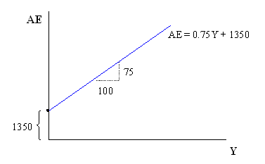
It is this equation that weĺll use to represent aggregate expenditures. On a graph, we have something that looks very similar to the consumption equation graph above. The AE graph appears as follows:

We want to make note of a couple things. First, the mpc is the slope of the consumption
function (equation) and the slope of the AE equation. This is true because we have assumed
that so many of our expenditure categories are autonomous. One impact of moving closer
toward reality (i.e. by not assuming so many variables are autonomous) is that the slope
of this graph changes. The mpc remains the slope of the consumption function, but becomes
only a part of the slope of the AE equation.
A second thing to note is that even though we have an equation for AE, we donĺt know the
exactly how much will be spent. That is, we donĺt know the equilibrium values of AE and Y.
This requires doing some further work, something weĺll save for another handout.